Numpy เบื้องต้น - 1D

30 minutes

วัตถุประสงค์

หลังจากทำทำแล็บ นศ.จะสามารถ

• Import ไลบรารี่ (Library) numpy และใช้งานไลบรารี่เบื้องต้นได้

• ดำเนินการทางคณิตศาสตร์กับข้อมูล NumPy arrays (อาร์เรย์ 1 มิติ) ได้

• Import ไลบรารี่ (Library) matplotlib และพล็อตกราฟอย่างง่ายได้

Ref:

• https://docs.scipy.org/doc/numpy/user/quickstart.html

• https://docs.scipy.org/doc/numpy/user/basics.html

---

import ไลบรารี่ NumPy

หนึ่งในจุดเด่นของภาษาไพธอนคือ มีไลบรารีเสริมมากมายครอบคลุมการใช้งานที่หลากหลาย

ในบรรดาไลบรารีต่างๆ numpy และ matplotlib เป็น 2 ไลบรารีที่มีความสำคัญและใช้กันอย่างแพร่หลายที่สุด

เรามักจะใช้ numpy คำนวณและวิเคราะห์ข้อมูลเชิงตัวเลข จากนั้นนำข้อมูลออกมาแสดงผลเป็นกราฟและแผนภาพต่างๆ ให้เห็นภาพชัดเจนยิ่งขึ้นโดยใช้ matplotlib

(หากใช้ไลบรารี numpy + matplotlib + scipy จะทำให้ไพธอนทัดเทียมกับโปรแกรม matlab (แมตแล็บ) โดยที่ไม่ต้องเสียค่าใช้จ่าย และเมื่อใช้ร่วมกับไลบรารี pandas + scikit-learn + ฯลฯ ก็จะทำให้ไพธอนเหนือกว่า matlab ขึ้นไปอีก)

การ Import ไลบรารี่

• แบบที่ 1: import <library_name> as <alias_name>

• แบบที่ 2: import <library_name>

• แบบที่ 3: from <library_name> import <variable(sub_module/sub_package/method)>
              from <library_name> import <variable(sub_module/sub_package/method)> as <alias_name>

• แบบที่ 4: from <library_name> import *

# Import the libraries

import time 
import sys
import numpy as np # To define an alias for an imported module

# import the pyplot module of the matplotlib library under the alias plt.
import matplotlib.pyplot as plt
%matplotlib inline  

# Plotting functions using matplotlib

def Plotvec1(u, z, v):
    
    ax = plt.axes() # Creating a new full window axes
    ax.arrow(0, 0, *u, head_width=0.1, color='r', head_length=0.1) # Axes.arrow(x, y, dx, dy, **kwargs)[source] : This draws an arrow from (x, y) to (x+dx, y+dy)
    plt.text(*(u + 0.1), 'u') # matplotlib.pyplot.text(x, y, s, fontdict=None, **kwargs)[source] : Add the text s to the Axes at location x, y in data coordinates.
    ax.arrow(0, 0, *v, head_width=0.1, color='b', head_length=0.1)
    plt.text(*(v + 0.1), 'v')
    ax.arrow(0, 0, *z, head_width=0.1, head_length=0.1)
    plt.text(*(z + 0.1), 'z')
    #plt.ylim(-2, 2) # Fixed Y-scale
    #plt.xlim(-2, 2) # Fixed X-scale
    ax.autoscale()  # Auto-scale
    ax.set_aspect('equal')

def Plotvec2(a,b):
    ax = plt.axes() # Creating a new full window axes
    ax.arrow(0, 0, *a, head_width=0.1, color ='r', head_length=0.1)
    plt.text(*(a + 0.1), 'a')
    ax.arrow(0, 0, *b, head_width=0.1, color ='b', head_length=0.1)
    plt.text(*(b + 0.1), 'b')
    plt.ylim(-2, 2)
    #plt.ylim(-2, 2)
    #plt.xlim(-2, 2)   
    ax.autoscale()  # Auto-scale
    ax.set_aspect('equal')

สร้างลิสต์ (List) ขึ้นมา

# Create a python list using square brackets.
a = ["0", 1, "two", "3", 4]

เราสามารถเข้าถึงสมาชิกภายในได้โดยใช้ index

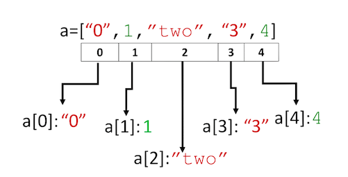
เข้าถึงสมาชิกแต่ละตัวในลิสต์โดยใช้เครื่องหมายวงเล็บเหลี่ยม [ ] (square brackets) ดังนี้

# Print each element

print("a[0]:", a[0])
print("a[1]:", a[1])
print("a[2]:", a[2])
print("a[3]:", a[3])
print("a[4]:", a[4])

a[0]: 0
a[1]: 1
a[2]: two
a[3]: 3
a[4]: 4

ลิสต์ไม่ได้ถูกทำมาเพื่อใช้ในการคำนวณโดยเฉพาะ ทำให้ไม่สามารถคำนวณได้โดยตรง หากเราต้องการจะนำอาร์เรย์มาบวกลบหรือทำอะไรก็ตาม จะพบว่าผลลัพธ์ไม่เป็นไปอย่างที่ต้องการ

เราลองสร้าง List ขึ้นมาสองตัวแปร x และ y

x = [0, 1, 2, 3, 4]
y = [9, 8, 7, 6, 5]

print(x+y)

[0, 1, 2, 3, 4, 9, 8, 7, 6, 5]

ผลที่ได้ไม่ใช่การนำอาร์เรย์มาบวกกัน ซึ่งผลควรจะได้เป็น [9, 9, 9, 9, 9] แต่กลับกลายเป็นการเอามาต่อกัน

หากต้องการให้บวกเมทริกซ์จะต้องทำการวนซ้ำเพื่อให้มีการคำนวณที่ตัวส่วนประกอบแต่ละตัว

#z = [0, 0, 0, 0, 0]
z = [0 for i in x]

for i in range(len(x)):
    z[i] = x[i]+y[i]
print(z) 

[9, 9, 9, 9, 9]

จะเห็นว่ามีความยุ่งยาก หากสามารถทำให้เขียนแค่ x+y แล้วบวกกันได้เลย ชีวิตก็คงจะง่ายขึ้น!

สิ่งที่จะตอบโจทย์นี้ได้ก็คือ numpy นั่นเอง

ถ้า x และ y ไม่ใช่ลิสต์แต่เป็นออบเจ็กต์ ndarray ของ numpy แล้วละก็ x+y ก็จะเป็นการบวกอาร์เรย์ทันที นี่คือความสะดวกของ numpy

แต่ไม่ใช่แค่นั้น นอกจากจะทำให้เขียนโค้ดสะดวกขึ้นแล้ว ยังทำให้การคำนวณเร็วขึ้นมากด้วย

ไพธอนเป็นภาษาที่ถูกออกแบบมาเพื่อให้เขียนง่ายต่อการเขียนและมีความยืดหยุ่นสูง แต่ก็มีข้อเสียคือทำงานช้าเมื่อเทียบกับภาษาระดับที่สูงไม่มากอย่างภาษา C หรือ Fortan

numpy เป็นไลบรารีที่มีเบื้องหลังการทำงานเป็นภาษาซี ดังนั้นจึงมีความเร็วสูงในการคำนวณมากกว่า

---

NumPy คืออะไร?

NumPy (Numerical Python) เป็นไลบรารีที่สำคัญมากที่สุดในไพธอนเลยก็ว่าได้ เนื่องจากใช้สำหรับการคำนวณทางคณิตศาสตร์ที่ซับซ้อนได้อย่างมีประสิทธิภาพ เช่นการเขียนชุดตัวเลขให้อยู่ในรูปแมทริกซ์ ซึ่งทำให้สะดวกต่อการเขียนโค้ดและการคำนวณอย่างมากมาก

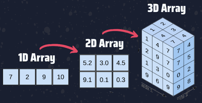
NumPy มีออบเจ็กต์พิเศษชนิดหนึ่งที่ชื่อว่า ndarray (N-d Array; N-dimensional array (multidimensional, homogeneous array)) ซึ่งเป็นออบเจ็กต์ที่เก็บข้อมูลเป็นกลุ่มเป็นแถว สามารถเก็บเป็นหลายมิติได้และสามารถนำข้อมูลภายในมาคำนวณได้อย่างรวดเร็ว

อาร์เรย์ (Arrays) เป็นคุณสมบัติหลักของ NumPy NumPy Arrays มีลักษณะคล้ายกับ List (เก็บข้อมูลเป็นชุดของข้อมูลที่มีลำดับของข้อมูล) ยกเว้น สมาชิกทุกตัวในอาร์เรย์จะต้องเป็นข้อมูลชนิดเดียวกัน โดยทั่วไปแล้วข้อมูลที่เก็บในอาร์เรย์จะเป็นตัวเลขเช่น int หรือ float

เนื่องจาก NumPy เป็นไลบรารี่ 3rd-party จึงต้องติดตั้งก่อนใช้งาน และตอนเขียนโค้ดต้อง import ไลบรารี่ก่อน

# Let’s install the Numpy library
# !pip install numpy

# import numpy library


import numpy as np 

เวลาที่เรียกชื่อฟังก์ชันต่างๆใน Numpy จะเรียกโดยขึ้นต้นด้วย np.

”Module”, “Package”, “Library” ??

Module (โมดูล) คือ Python File (.py files) ที่เก็บฟังก์ชั่น คลาสต่างๆ และตัวแปรโกบอลที่ใช้เป็นตัวชี้บ่งสถานะ (Flag). ตัวอย่างของโมดูล เช่น math

Package (แพ็คเกจ) ก็คือ โฟลเดอร์ (Folder/Directory) ที่เก็บไพธอนโมดูลต่างๆ โดยภายในแพ็คเกจจะมีไฟล์ init.py กำหนดไว้ในโฟลเดอร์ เพื่อบ่งบอกว่าเป็นโฟลเดอร์ของแพ็คเกจ (ไฟล์นี้สามารถเป็นไฟล์ว่าง (Empty file) ได้) ตัวอย่างของแพ็คเกจ เช่น numpy, Requests, Matplotlib

Library (ไลบรารี) คือ แพ็คเกจต่างๆ ที่ถูกรวบรวมไว้ โดยทั่วไปแล้ว ไพธอนแพ็คเกจกับไพธอนไลบรารีไม่ต่างกัน

การสร้างชุดข้อมูลอาร์เรย์ (1D Numpy Array)

การสร้างอาเรย์มีอยู่หลายวิธี แต่วิธีที่พื้นฐานที่สุดคือสร้างขึ้นมาจาก List, Tuple หรือ Range โดยใช้ np.array

เราลองเปลี่ยนชุดข้อมูล List ข้างต้นให้เป็นอาร์เรย์

help(np.array)

Help on built-in function array in module numpy:

array(...)
    array(object, dtype=None, *, copy=True, order='K', subok=False, ndmin=0,
          like=None)
    
    Create an array.
    
    Parameters
    ----------
    object : array_like
        An array, any object exposing the array interface, an object whose
        __array__ method returns an array, or any (nested) sequence.
        If object is a scalar, a 0-dimensional array containing object is
        returned.
    dtype : data-type, optional
        The desired data-type for the array.  If not given, then the type will
        be determined as the minimum type required to hold the objects in the
        sequence.
    copy : bool, optional
        If true (default), then the object is copied.  Otherwise, a copy will
        only be made if __array__ returns a copy, if obj is a nested sequence,
        or if a copy is needed to satisfy any of the other requirements
        (`dtype`, `order`, etc.).
    order : {'K', 'A', 'C', 'F'}, optional
        Specify the memory layout of the array. If object is not an array, the
        newly created array will be in C order (row major) unless 'F' is
        specified, in which case it will be in Fortran order (column major).
        If object is an array the following holds.
    
        ===== ========= ===================================================
        order  no copy                     copy=True
        ===== ========= ===================================================
        'K'   unchanged F & C order preserved, otherwise most similar order
        'A'   unchanged F order if input is F and not C, otherwise C order
        'C'   C order   C order
        'F'   F order   F order
        ===== ========= ===================================================
    
        When ``copy=False`` and a copy is made for other reasons, the result is
        the same as if ``copy=True``, with some exceptions for 'A', see the
        Notes section. The default order is 'K'.
    subok : bool, optional
        If True, then sub-classes will be passed-through, otherwise
        the returned array will be forced to be a base-class array (default).
    ndmin : int, optional
        Specifies the minimum number of dimensions that the resulting
        array should have.  Ones will be prepended to the shape as
        needed to meet this requirement.
    like : array_like, optional
        Reference object to allow the creation of arrays which are not
        NumPy arrays. If an array-like passed in as ``like`` supports
        the ``__array_function__`` protocol, the result will be defined
        by it. In this case, it ensures the creation of an array object
        compatible with that passed in via this argument.
    
        .. versionadded:: 1.20.0
    
    Returns
    -------
    out : ndarray
        An array object satisfying the specified requirements.
    
    See Also
    --------
    empty_like : Return an empty array with shape and type of input.
    ones_like : Return an array of ones with shape and type of input.
    zeros_like : Return an array of zeros with shape and type of input.
    full_like : Return a new array with shape of input filled with value.
    empty : Return a new uninitialized array.
    ones : Return a new array setting values to one.
    zeros : Return a new array setting values to zero.
    full : Return a new array of given shape filled with value.
    
    
    Notes
    -----
    When order is 'A' and `object` is an array in neither 'C' nor 'F' order,
    and a copy is forced by a change in dtype, then the order of the result is
    not necessarily 'C' as expected. This is likely a bug.
    
    Examples
    --------
    >>> np.array([1, 2, 3])
    array([1, 2, 3])
    
    Upcasting:
    
    >>> np.array([1, 2, 3.0])
    array([ 1.,  2.,  3.])
    
    More than one dimension:
    
    >>> np.array([[1, 2], [3, 4]])
    array([[1, 2],
           [3, 4]])
    
    Minimum dimensions 2:
    
    >>> np.array([1, 2, 3], ndmin=2)
    array([[1, 2, 3]])
    
    Type provided:
    
    >>> np.array([1, 2, 3], dtype=complex)
    array([ 1.+0.j,  2.+0.j,  3.+0.j])
    
    Data-type consisting of more than one element:
    
    >>> x = np.array([(1,2),(3,4)],dtype=[('a','<i4'),('b','<i4')])
    >>> x['a']
    array([1, 3])
    
    Creating an array from sub-classes:
    
    >>> np.array(np.mat('1 2; 3 4'))
    array([[1, 2],
           [3, 4]])
    
    >>> np.array(np.mat('1 2; 3 4'), subok=True)
    matrix([[1, 2],
            [3, 4]])

Syntax ของการสร้างชุดข้อมูลอาร์เรย์ (nampy.array Syntax)

np.array(object, dtype=None)

# Create a numpy array (integer array)

np.array([0, 1, 2, 3, 4])

array([0, 1, 2, 3, 4])

# Create a numpy array

a = np.array([0, 1, 2, 3, 4])
a

array([0, 1, 2, 3, 4])

สมาชิกแต่ละตัวในอาร์เรย์ต้องเป็นข้อมูลชนิดเดียวกัน ในกรณีคือ int

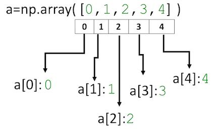
เช่นเดียวกับ List เราสามารถเข้าถึงข้อมูลภายในโดยอ้างถึงหมายเลขดัชนี (index) ผ่านเครื่องหมายวงเล็บเหลี่ยม [ ] (square brackets)

# Print each element

print("a[0]:", a[0])
print("a[1]:", a[1])
print("a[2]:", a[2])
print("a[3]:", a[3])
print("a[4]:", a[4])

a[0]: 0
a[1]: 1
a[2]: 2
a[3]: 3
a[4]: 4

เราสามารถเข้าถึงสมาชิกทีละหลายๆ ตัวได้ด้วยการใช้โคลอน : เช่นเดียวกับลิสต์

print(a[0:3])

[0 1 2]

หากมี : เพิ่มมาอีกตัว แล้ววางตัวเลขไว้ทางขวาของ : จะเป็นการกำหนดระยะเว้นช่วง (เหมือน List)

print(a[::2])

[0 2 4]

และหากใส่เลขติดลบ ก็จะกลายเป็นการไล่ถอยหลัง (เหมือน List)

print(a[::-2])

[4 2 0]

จะเห็นว่า หากต้องการกลับลำดับสมาชิกในอาเรย์ทั้งหมด (เรียงจากหลังไปหน้า) ก็แค่ใส่ [::-1] ไปเท่านั้น เป็นการใช้งานที่สะดวกมาก

# Reverse
print(a[::-1])

[4 3 2 1 0]

np.array([1, 4, 2, 5, 3])

array([1, 4, 2, 5, 3])

เราสามารถสร้างอาเรย์โดยใช้ List Comprehension ได้ เช่น

# nested lists result in 1-dimensional array
np.array([i*2 for i in range(10)])

array([ 0,  2,  4,  6,  8, 10, 12, 14, 16, 18])

a = np.array([i*i for i in range(50) if i%2!=1])
a

array([   0,    4,   16,   36,   64,  100,  144,  196,  256,  324,  400,
        484,  576,  676,  784,  900, 1024, 1156, 1296, 1444, 1600, 1764,
       1936, 2116, 2304])

NumPy arange() เป็นอีกวิธีหนึ่งในการสร้าง array (เรียกว่า NumPy routines สำหรับสร้าง array) โดยมี

Syntax:

numpy.arange(start, stop, step, dtype)

โดย dtype คือ ชนิดข้อมูลของสมาชิกใน array หากไม่ระบุจะประเมินให้อัตโนมัติโดยพิจารณาจากชนิดข้อมูล start stop และ step

# Create an array filled with a linear sequence
# Starting at 0, ending at 20, stepping by 2
# (this is similar to the built-in range() function)
np.arange(0, 20, 2)

array([ 0,  2,  4,  6,  8, 10, 12, 14, 16, 18])

# Boolean Indexing
# We can also set conditionals inside square brackets to filter elements out.
q = np.arange(0, 20, 2)
q[q<10]

array([0, 2, 4, 6, 8])

สิ่งที่แตกต่างระหว่าง NumPy arange() กับฟังก์ชั่น range() อีกอย่างก็คือ NumPy arange() สามารถเป็นเลขชุดทศนิยมได้ ในขณะที่ range() เป็นเฉพาะจำนวนเต็มเท่านั้น

for i in np.arange(0, 10, 2.5):
    print(i)

0.0
2.5
5.0
7.5

for i in range(0,10, 2):
    print(i)

0
2
4
6
8

ชนิดของข้อมูลในอาร์เรย์

ถ้าเราตรวจสอบชนิดของข้อมูล จะพบว่าเป็นชนิด (ออบเจ็กต์) numpy.ndarray (N-d Array; N-dimensional array (multidimensional, homogeneous array))

# Check the type of the array

type(a)

numpy.ndarray

สมาชิกทุกตัวในอาร์เรย์ต้องเป็นข้อมูลชนิดเดียวกัน เราสามารถตรวจสอบชนิดของข้อมูลที่เก็บในอาร์เรย์ได้โดยเรียกแอตทริบิวต์ (attribute) dtype ในกรณีนี้เป็นชนิดจำนวนเต็ม 64-bit)

# Check the type of the values stored in numpy array

a.dtype

dtype('int64')

ตอนสร้างสร้างอาร์เรย์ หากมีสมาชิกที่มีทศนิยมแม้แต่ตัวเดียวทั้งหมดก็จะกลายเป็น float64 ทันที

# Create a numpy array with real numbers 

b = np.array([0, 1, 2, 3, 4, 3.14])
b

array([0.  , 1.  , 2.  , 3.  , 4.  , 3.14])

# Create a numpy array with real numbers 

b = np.array([0, 1, 2, 3, 4, 3.14159265359])
b

array([0.        , 1.        , 2.        , 3.        , 4.        ,
       3.14159265])

จะเห็นว่าข้อมูลในอาเรย์จะต้องเป็นข้อมูลที่มีชนิดเดียวกันและมีขนาดเท่ากันหมดทุกตัว หากตอนที่สร้างอาเรย์มีสมาชิกที่ชนิดต่างกันจะถูกทำให้เหมือนกันหมด!

ถ้าเราตรวจสอบชนิดของข้อมูล จะพบว่าเป็นชนิด numpy.ndarray

# Check the type of array

type(b)

numpy.ndarray

เราสามารถตรวจสอบชนิดของข้อมูลโดยเรียกแอตทริบิวต์ (attribute) dtype ในกรณีนี้เป็นชนิด float 64 ไม่ใช่จำนวนเต็ม

# Check the value type

b.dtype

dtype('float64')

การกำหนดค่าใหม่ให้กับอาร์เรย์ (เขียนทับข้อมูล)

เช่นเดียวกับ List เราสามารถเปลี่ยนค่าอาร์เรย์เมื่อไหร่ก็ได้โดยการใส่ค่าใหม่ทับลงไป

ตัวอย่าง เราสร้างอาร์เรย์ c ขึ้นมาก่อนโดยใช้ลิสต์

# Create numpy array

c = np.array([20, 1, 2, 3, 4])
c

array([20,  1,  2,  3,  4])

เราสามารถเปลี่ยนค่าของสมาชิกตัวแรกให้เป็น 100

# Assign the first element to 100

c[0] = 100
c

array([100,   1,   2,   3,   4])

เราสามารถเปลี่ยนสมาชิกตัวสุดท้ายให้มีค่าเป็น 0 ได้โดยใช้ดัชนีเชิงลบ (Negative indexing) เหมือนกับ List

# Assign the last element to 0

c[-1] = 100
c

array([100,   1,   2,   3, 100])

เราสามารถกำหนดค่าให้กับสมาชิกมากกว่าหนึ่งตัวได้โดยระบุช่วงของข้อมูล ดังนี้ (ทำได้เหมือนกับ List)

# Set the fourth element and fifth element to 300 and 400

c[3:5] = 300, 400
c

array([100,   1,   2, 300, 400])

หากต้องการเปลี่ยนค่าของสมาชิกทุกตัวให้เป็น 100 ก็สามารถทำได้ (List ใชรูปแบบคำสั่งแบบนี้ทำไม่ได้)

c[:] = 100
c

array([100, 100, 100, 100, 100])

การกำหนดค่าด้วยลิสต์ดัชนี (Integer array indexing)

# Recreate numpy array

c = np.array([0, 1, 2, 3, 4])
c

array([0, 1, 2, 3, 4])

เราสามารถใช้ลิสต์เป็นดัชนีเพื่อกำหนดเฉพาะดัชนีที่ต้องการได้

เราจะสร้างลิสต์ select ขึ้นมา ซึ่งภายในมีเลขดัชนีหลายค่า

# Create the index list

select = [0, 2, 4]

เราสามารถใช้ลิสต์ดัชนีเป็นอาร์กิวเมนต์ในวงเล็บสี่เหลี่ยมได้

# Use List to select elements

d = c[select]
d

array([0, 2, 4])

c[[0, 2, 4]]

array([0, 2, 4])

นอกจากนี้ยังสามารถใช้ลิสต์ดัชนีแก้ไขค่าของสมาชิกได้อีกด้วย ยกตัวอย่างเช่น เปลี่ยนค่าเป็น 100000

# Assign the specified elements to new value

c[select] = 100000
c

array([100000,      1, 100000,      3, 100000])

# c[0, 2, 4] = 0
c[[0, 2, 4]] = 0
c

array([0, 1, 0, 3, 0])

แอตทริบิวต์และเมธอดอื่นๆ ของอาร์เรย์

นอกจากแอตทริบิวต์ dtype แล้ว ยังมีแอตทริบิวต์อื่นๆ อีกที่สามารถให้ข้อมูลของตัวอาเรย์นั้นๆ ได้ เช่น

size จำนวนสมาชิกในอาเรย์, ndim จำนวนมิติของอาเรย์, shape รูปร่างของอาเรย์

เราจะเรียนรู้แอตทริบิวต์อื่นๆ ของอาร์เรย์โดยผ่านอาร์เรย์ a

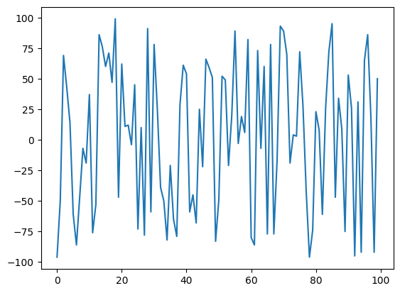
ก่อนอื่น สร้างอาร์เรย์ a เลขจำนวนเต็ม จำนวน 100 ตัวเลข โดยการเรียกใช้ฟังก์ชั่น randint()

ฟังก์ชั่น randint() ใช้สุ่ม (Random) ตัวเลขจำนวนเต็ม โดยจะทำการสุ่มจำนวนเต็มที่อยู่ในช่วงที่กำหนด (low - high) ออกมาตามจำนวน size ที่กำหนด

numpy.random.randint(low, high=None, size=None, dtype=int)

a = np.random.randint(-100,100,100)
a

array([-96, -50,  69,  43,  14, -61, -86, -47,  -7, -19,  37, -76, -53,
        86,  76,  60,  71,  47,  99, -47,  62,  11,  12,  -4,  45, -73,
        10, -78,  91, -59,  78,  25, -39, -50, -82, -21, -65, -79,  29,
        61,  54, -59, -45, -68,  25, -22,  66,  59,  51, -83, -49,  52,
        49, -21,  20,  89,  -3,  19,   6,  82, -80, -86,  73,  -7,  60,
       -77,  78, -77, -17,  93,  89,  70, -19,   4,   3,  72,  28, -42,
       -96, -74,  23,   8, -61,  26,  72,  95, -47,  34,   9, -75,  53,
        26, -95,  31, -92,  65,  86,  18, -92,  50])

ดูข้อมูลกันก่อน โดยการพล็อตกราฟอย่างง่าย

plt.plot(a)

[<matplotlib.lines.Line2D at 0x11d1f9580>]

แอตทริบิวต์ size จำนวนสมาชิกในอาร์เรย์

# Get the size of numpy array

a.size

100

ndim (number of dimensions) จำนวนมิติของอาเรย์

# Get the number of dimensions of numpy array

a.ndim

1

shape รูปร่างของอาเรย์ (จำนวนสามาชิกในแต่ละมิติ (dimension))

ตอนนี้อาร์เรย์ที่สร้างขึ้นเป็นแค่ 1 มิติ

# Get the shape/size of numpy array

a.shape

(100,)

แค่ถ้าเป็นอาร์เรย์ที่สร้างขึ้นเป็น 2 มิติ (2-dimension)

k = np.array([[1,2,3],
              [4,5,6],
              [7,8,9]    
    ])

k.ndim

2

k.shape

(3, 3)

NumPy ยังมีเมธอด (Method) สำหรับการคำนวณค่าทางสถิติสำหรับชุดข้อมูลที่เก็บในอาร์เรย์ เช่น Mean, Max, Min, SD (Standard deviation) และ Var โดยเรียกด้วย mean(), max(), min(), std() และ var() ตามลำดับ เป็นต้น

ค่าเฉลี่ย (Mean) คือ ค่ากลางที่ได้จากการนำเอาข้อมูลแต่ละตัวมารวมกัน แล้วนำผลรวมที่ได้มาหารด้วยจำนวนข้อมูลทั้งหมด

ส่วนเบี่ยงเบนมาตรฐาน (SD; Standard Deviation) คือ ค่ารากที่สองของผลรวมของความแตกต่างระหว่างข้อมูลดิบกับค่าเฉลี่ยยกกำลังสอง (sum of squares ของผลต่าง) หารด้วยจำนวนข้อมูลทั้งหมด

ค่าความแปรปรวน (Variance) คือ ค่าที่คำนวณมาจาก ค่าเบี่ยงเบนมาตรฐาน หรือ ส่วนเบี่ยงเบนมาตรฐาน ยกกำลัง 2

ค่าสูงสุด (max) ค่าต่ำสุด (min)

# Get the biggest value in the numpy array

max_a = a.max()
max_a

99

# Get the smallest value in the numpy array

min_a = a.min()
min_a

-96

ค่าเฉลี่ย (Mean)

ถ้าหาแบบ Manual ค่าเฉลี่ย (Mean) จะสามารถหาได้จาก ผลรวมทั้งหมด/จำนวน

# Cal by manual
sum_a = a[0]+a[1]+a[2]+a[3]+a[4] # +... หมดแรงก่อน 
sum_a

-20

sum_a = 0
for n in a:
    sum_a += n
sum_a

285

ใช้คำสั่งที่สั้นกว่านั้น

sum_a = sum(a[:])
sum_a

285

แต่ถ้าใช้ Numpy

# numpy.ndarray.sum: Return the sum of the array elements over the given axis.
sum_a = a.sum()
sum_a

285

หาค่าเฉลี่ย (Mean) จาก ผลรวมทั้งหมด/จำนวน

# Cal by manual
mean_a = sum_a/a.shape[0]
mean_a

2.85

แต่ถ้าใช้ Numpy

# Get the mean of numpy array

mean_a = a.mean()
mean_a

2.85

ค่าเบี่ยงเบนมาตรฐาน (Standard deviation)

# Get the standard deviation of numpy array

std_a=a.std()
std_a

59.41874704165345

ค่าความแปรปรวน (Variance)

# Get the smallest value in the numpy array

var_a = a.var()
var_a

3530.5875000000005

นอกจากการเรียกใช้เมธอดแล้ว เรายังสามารถเรียกใช้งานในรูปแบบฟังก์ชันก็ได้ (ใช้ชื่อฟังก์ชั่นเหมือนกับชื่อเมธอด) เช่น

np.var(a)

3530.5875000000005

np.floor(b)

array([0., 1., 2., 3., 4., 3.])

ตัวดำเนินการสำหรับ Numpy Array

เมื่อใช้ตัวดำเนินการทางคณิตศาสต์กับอาร์เรย์แล้ว จะได้ ndarray ชุดใหม่เสมอ

การบวกลบอาร์เรย์

พิจารณา Numpy Array u

u = np.array([2, 1])
u

array([2, 1])

พิจารณา Numpy Array v

v = np.array([1, 2])
v

array([1, 2])

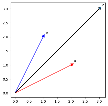
เราสามารถบวกอาร์เรย์ทั้งสองนี้แล้วกำหนดให้เป็นอาร์เรย์ z

# Numpy Array Addition
# To add two or more arrays use np.add(a,b) or the + sign.

#z = np.add(u, v)
z = u + v
z

array([3, 3])

การดำเนินข้างต้นเทียบเท่ากับการบวกเวกเตอร์

# Plot numpy arrays

Plotvec1(u, z, v)

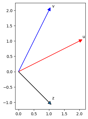
การลบก็เช่นเดียวกัน

# To subtract one array from another use the np.subtract(a,b) or the — sign
#z = np.subtract(u, v)
z = u - v
z

array([ 1, -1])

Plotvec1(u, z, v)

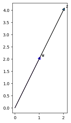
การคูณอาร์เรย์ (Multiplication) ด้วยสเกลาร์

พิจารณา Numpy Array y

# Create a numpy array

y = np.array([1, 2])
y

array([1, 2])

เราสามารถคูณสมาชิกทุกตัวในอาร์เรย์ด้วย 2 ได้เลยโดยที่ไม่ต้องใช้คำสั่งลูป

# Numpy Array Multiplication
# To multiply array by scalar use np.multiply(a,b)or the * sign.

#z = np.multiply(2, y)
z = 2 * y

z

array([2, 4])

การดำเนินข้างต้นเทียบเท่ากับการคูณเวกเตอร์ด้วยสเกลาร์

Plotvec1(y, z, y)

การคูณสองอาร์เรย์ (Product)

พิจารณา Numpy Array u

# Create a numpy array

u = np.array([1, 2])
u

array([1, 2])

พิจารณา Numpy Array v

# Create a numpy array

v = np.array([3, 2])
v

array([3, 2])

การคูณอาร์เรย์สองอาร์เรย์ u และ v จะได้

# Calculate the production of two numpy arrays
# To multiply two arrays use np.multiply(a,b)or the * sign.

#z = np.multiply(u, v)
z = u * v
z

array([3, 4])

ซึ่งเป็นการคูณแต่ละสมาชิกที่อยู่ในตำแหน่งเดียวกันเป็นคู่ๆ (element-by-element)

นอกจากการคูณแล้ว การหาร การยกกำลัง และหารเอาเศษ ก็เป็นการคำนวณเป็นคู่ๆ ทีละตัว ดังตัวอย่างต่อไปนี้

# To divide two arrays usenp.divide(a,b)or the / sign.
print(u/v, '\n')

print(u**v, '\n')
print(u%v, '\n')

[0.33333333 1.        ] 

[1 4] 

[1 0] 

การคูณแบบ Dot Product

ถ้าต้องการคูณสองอาร์เรย์แบบ Dot Product ระหว่าง u และ v ใช้ฟังก์ชั่น dot() หรือใช้โอเปอร์เรเตอร์ @

# Calculate the dot product
u = np.array([1, 2])
v = np.array([3, 2])

np.dot(u, v)

7

u@v

7

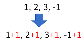
การบวกและลบอาร์เรย์ด้วยค่าคงที่

พิจารณา Numpy Array ต่อไปนี้

# Create a constant to numpy array

u = np.array([1, 2, 3, -1]) 
u

array([ 1,  2,  3, -1])

บวกค่าคงที่ 1 ให้กับแต่ละสมาชิกที่อยู่ในอาร์เรย์

# Add the constant to array

u + 1

array([2, 3, 4, 0])

สิ่งที่เกิดขึ้นสรุปเป็นรูปภาพได้ดังรูปต่อไปนี้

ฟังก์ชั่นทางคณิตศาสตร์

ค่าของ \(\pi\) (Pi) ใน Numpy

# The value of pi

np.pi

3.141592653589793

เราสามารถสร้างอาร์เรย์ในหน่วยเรเดียน

# Create the numpy array in radians

x = np.array([0, np.pi/2 , np.pi])
x

array([0.        , 1.57079633, 3.14159265])

เราสามารถใช้ฟังก์ชัน sin กับอาร์เรย์ x และให้ผลลัพท์เป็นอาร์เรย์ y ซึ่งเป็นการหาค่าไซน์ของสมาชิกทุกตัวในอาร์เรย์ x

# Calculate the sin of each elements

y = np.sin(x)
y

array([0.0000000e+00, 1.0000000e+00, 1.2246468e-16])

# ใช้ฟังก์ชั่น np.radians()
x = np.array([0, np.radians(90) , np.radians(180)])
y = np.sin(x)
y

array([0.0000000e+00, 1.0000000e+00, 1.2246468e-16])

จากผลข้างต้น เราจพพบว่า sin(𝜋) ≠ 0 เนื่องจากไม่มีตัวเลขทศนิยมที่จะมาแทนค่า 𝜋 จริงๆ ได้ แก้ด้วยการประมาณค่าโดยใช้ฟังก์ชัน np.around()

np.around(y, decimals=5)

array([0., 1., 0.])

ค่าคงที่ที่สำคัญอื่นๆ ใน numpy

np.e
np.pi
np.nan
np.inf

นอกจากการคำนวณพื้นฐานแล้ว numpy ยังมีฟังก์ชันสำหรับคำนวณที่ใกล้เคียงกับในไลบรารี math เช่น abs, sqrt, log, log10, exp, sin, cos, tan, arcsin, arccos, arctan, sinh, cosh, tanh, arcsinh, arccosh, arctanh

z = np.sqrt(x)
z

array([0.        , 1.25331414, 1.77245385])

ฟังก์ชัน numpy.linspace (start, stop, n)

ฟังก์ชั่นที่ใช้สร้างอาร์เรย์ใน NumPy อีกฟังก์ชั่น คือ ฟังก์ชั่น numpy.linspace() ฟังก์ชั่นนี้คล้ายกับฟังก์ชั่น numpy.arange( ) แต่จะแทนที่จะระบุ step (ระยะห่างของข้อมูลแต่ละตัว) ฟังก์ชั่น numpy.linspace() จะระบุเป็นจำนวนของข้อมูลที่ต้องการ โดยระยะห่างของข้อมูลแต่ละตัวจะถูกปรับให้มีขนาดเท่าๆ กันโดยอัตโนมัติ มักใช้กำหนดข้อมูลในการพล็อตกราฟ

Syntax

numpy.linspace(start, stop, num)

ความหมายของแต่ละพารามิเตอร์:

start: ค่าเริ่มต้นของอาร์เรย์ stop: ค่าสุดท้ายของอาร์เรย์ num: จำนวนข้อมูลในอาร์เรย์ (default argument = 50)

np.linspace?

# Makeup a numpy array within [-2, 2] and 5 elements

np.linspace(-2, 2, num=5)

array([-2., -1.,  0.,  1.,  2.])

จาก -2 ถึง 2 แต่ต้องการ 9 จำนวน num=9

# Make a numpy array within [-2, 2] and 9 elements

np.linspace(-2, 2, num=9)

array([-2. , -1.5, -1. , -0.5,  0. ,  0.5,  1. ,  1.5,  2. ])

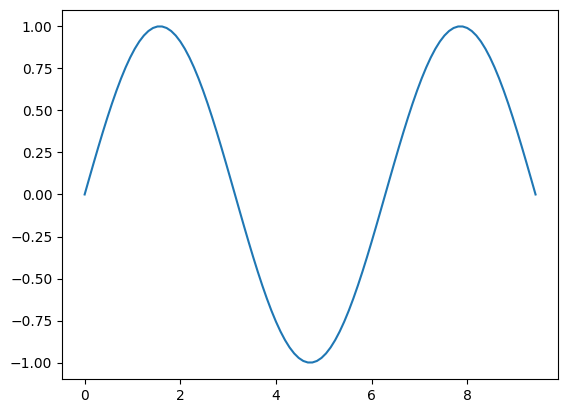
เราสามารถใช้ฟังก์ชั่น linspace() สร้างตัวเลข 100 จำนวนที่อยู่ในช่วงตั้งแต่ 0 ถึง \(3\pi\)

# Make a numpy array within [0, 3π] and 100 elements 

x = np.linspace(0, 3*np.pi, num=100)
x

array([0.        , 0.09519978, 0.19039955, 0.28559933, 0.38079911,
       0.47599889, 0.57119866, 0.66639844, 0.76159822, 0.856798  ,
       0.95199777, 1.04719755, 1.14239733, 1.23759711, 1.33279688,
       1.42799666, 1.52319644, 1.61839622, 1.71359599, 1.80879577,
       1.90399555, 1.99919533, 2.0943951 , 2.18959488, 2.28479466,
       2.37999443, 2.47519421, 2.57039399, 2.66559377, 2.76079354,
       2.85599332, 2.9511931 , 3.04639288, 3.14159265, 3.23679243,
       3.33199221, 3.42719199, 3.52239176, 3.61759154, 3.71279132,
       3.8079911 , 3.90319087, 3.99839065, 4.09359043, 4.1887902 ,
       4.28398998, 4.37918976, 4.47438954, 4.56958931, 4.66478909,
       4.75998887, 4.85518865, 4.95038842, 5.0455882 , 5.14078798,
       5.23598776, 5.33118753, 5.42638731, 5.52158709, 5.61678687,
       5.71198664, 5.80718642, 5.9023862 , 5.99758598, 6.09278575,
       6.18798553, 6.28318531, 6.37838508, 6.47358486, 6.56878464,
       6.66398442, 6.75918419, 6.85438397, 6.94958375, 7.04478353,
       7.1399833 , 7.23518308, 7.33038286, 7.42558264, 7.52078241,
       7.61598219, 7.71118197, 7.80638175, 7.90158152, 7.9967813 ,
       8.09198108, 8.18718085, 8.28238063, 8.37758041, 8.47278019,
       8.56797996, 8.66317974, 8.75837952, 8.8535793 , 8.94877907,
       9.04397885, 9.13917863, 9.23437841, 9.32957818, 9.42477796])

เราสมารถใช้ฟังก์ชั่น sin() หาค่า sine ของแต่ละสมาชิกในอาร์เรย์ x แล้วกำหนดค่าที่ได้เป็นอาร์เรย์ y

# Calculate the sine of x list

y = np.sin(x)

# Plot the result

plt.plot(x, y) # Plot y versus x as lines and/or markers using default line style and color
#plt.show() # Show graph

[<matplotlib.lines.Line2D at 0x11d37a940>]

เราสามารถกำหนดสี … และอื่นๆ เองได้

ดูรายละเอียดได้ที่ matplotlib.pyplot.plot

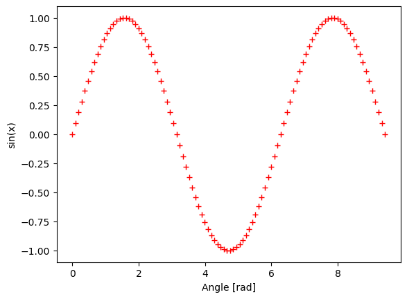
plt.plot(x, y, 'r+') # Plot with red plusses
plt.xlabel('Angle [rad]')
plt.ylabel('sin(x)')

Text(0, 0.5, 'sin(x)')

ตัวอย่างการพล็อตสัญญาณคลื่นสแควร์ (square wave) จากการรวม(ผลบวกของ) สัญญาณฮาร์โมนิกเลขคี่

สัญญาณรูปคลื่นที่ไม่ใช่สัญญาณไซน์ (Non-Sinusoidal Waveform) ที่เกิดขึ้นซ้ำๆ (มีคาบ มีความถี่ที่แน่นอน) สามารถสร้างขึ้นโดยการรวมแรงดันไฟกระแสตรง (DC) กับแรงดันคลื่นไซน์และ/หรือคลื่นโคไซน์ที่มีขนาดของสัญญาณหรือแอมพลิจูด (amplitude) และความถี่ (frequency) ที่แตกต่างกันเข้าด้วยกันได้

สัญญาณคลื่นสแควร์ (square wave) ประกอบด้วยสัญญาณรูปคลื่นไซน์ที่มีความถี่เดียวกันกับคลื่นสแควร์ (เรียกว่า สัญญาณที่ความถี่มูลฐานหรือสัญญาณฮาร์โมนิกลำดับที่-1 (Fundamental frequency or 1st order harmonic)) กับสัญญาณฮาร์โมนิกลำดับที่ 3,5 และ 7…(3rd, 5th, 7th order harmonic; เฉพาะฮาร์โมนิกเลขคี่) รวมเข้าด้วยกัน โดยที่แอมพลิจูดของฮาร์โมนิกเท่ากับ 1/N โดย N คือเลขฮาร์มอนิก (1, 3, 5, 7…)

ยกตัวอย่าง เช่น สัญญาณรูปคลื่นสแควร์ \(1V_{p-p}\) \(50Hz\) \(=\) สัญญาณรูปคลื่นไซน์ \(1V_{p-p}\) \(50Hz\) (ฮาร์มอนิกลำดับที่ 1) \(+\) สัญญาณรูปคลื่นไซน์ \(\frac{1}{3}V_{p-p}\) \(3*50Hz\) (ฮาร์มอนิกลำดับที่ 3) \(+\) สัญญาณรูปคลื่นไซน์ \(\frac{1}{5}V_{p-p}\) \(5*50Hz\) (ฮาร์มอนิกลำดับที่ 5) \(+\) สัญญาณรูปคลื่นไซน์ \(\frac{1}{7}V_{p-p}\) \(7*50Hz\) (ฮาร์มอนิกลำดับที่ 7) \(+ ...\)

ฮาร์มอนิก (Harmonic) คือ สัญญาณที่มีความถี่เป็นจำนวนเท่าของความถี่มูลฐาน (Fundamental Frequency) เช่น ความถี่มูลฐาน \(50 Hz\) ความถี่ฮาร์มอนิกลำดับที่ 3 จะเป็น \(150 (50*3)Hz\), ลำดับที่ 5 จะเป็น \(250 ((50*5))Hz\), ลำดับที่ 7 จะเป็น \(350 (50*7)Hz\) \(...\) เป็นต้น

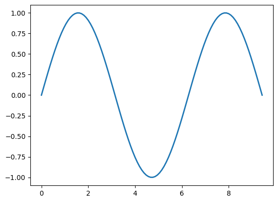
# first, third, fifth, seventh, and ninth harmonics.
h1 = np.sin(x)
h3 = np.sin(3*x)/3 
h5 = np.sin(5*x)/5 
h7 = np.sin(7*x)/7 
h9 = np.sin(9*x)/9


# Plot this fundamental frequency.
plt.plot(x, h1, linewidth=2) # plot with thick linewidth

[<matplotlib.lines.Line2D at 0x11d560f40>]

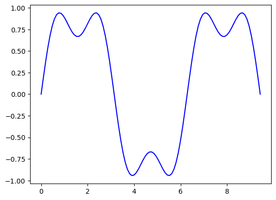
# Next add the third harmonic to the fundamental, and plot it.
plt.plot(x, h1+h3, 'b')
plt.plot()

[]

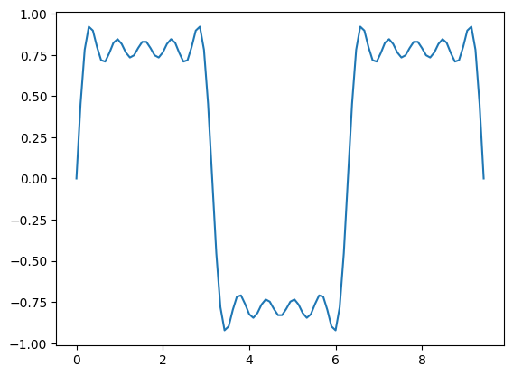
# Now use the first, third, fifth, seventh, and ninth harmonics.
plt.plot(x, h1+h3+h5+h7+h9)

[<matplotlib.lines.Line2D at 0x11d50a550>]

# Save graph ('eps', 'jpeg', 'jpg', 'pdf', 'png', 'ps', 'svg', 'svgz')
plt.savefig("sin.jpg")

<Figure size 640x480 with 0 Axes>

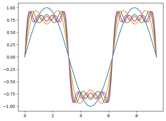
เราสามารถพล็อตหลายกราฟซ้อนกันได้

คำสั่ง plt.plot รันครั้งหนึ่งจะได้กราฟออกมาหนึ่งเส้น ถ้าหากสั่ง plt.plot ซ้ำก็จะได้เส้นกราฟออกมาอีกเส้น โดยสีของกราฟจะถูกกำหนดขึ้นโดยอัตโนมัติ ปกติแล้วเส้นแรกจะเป็นสีน้ำเงิน เส้นต่อมาเป็นสีส้ม แล้วก็สีเขียว แล้วก็เปลี่ยนเป็นสีอื่นไปอีกเรื่อยๆ

plt.plot(x, h1)
plt.plot(x, h1+h3)
plt.plot(x, h1+h3+h5)
plt.plot(x, h1+h3+h5+h7)
plt.plot(x, h1+h3+h5+h7+h9)

[<matplotlib.lines.Line2D at 0x11d34e280>]

plt.plot(x, h1+h3+h5+h7+h9)

[<matplotlib.lines.Line2D at 0x11d5f6100>]

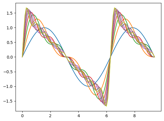
# sawtooth wave

h2 = np.sin(2*x)/2 
h4 = np.sin(4*x)/4 
h6 = np.sin(6*x)/6 
h8 = np.sin(8*x)/8


plt.plot(x, h1)
plt.plot(x, h1+h2)
plt.plot(x, h1+h2+h3)
plt.plot(x, h1+h2+h3+h4)
plt.plot(x, h1+h2+h3+h4+h5)
plt.plot(x, h1+h2+h3+h4+h5+h6)
plt.plot(x, h1+h2+h3+h4+h5+h6+h7)
plt.plot(x, h1+h2+h3+h4+h5+h6+h7+h8)
plt.plot(x, h1+h2+h3+h4+h5+h6+h7+h8+h9)

[<matplotlib.lines.Line2D at 0x11d661cd0>]

plt.plot(x, h1)

[<matplotlib.lines.Line2D at 0x11d6db730>]

นอกจากนี้ยังมีฟังก์ชันสำหรับเปลี่ยนหน่วยที่ใช้ในตรีโกณมิติ คือ deg2rad() หรือ radians() ใช้สำหรับเปลี่ยนจากองศาเป็นเรเดียน และ rad2deg() หรือ degrees() สำหรับเปลี่ยนจากเรเดียนเป็นองศา

---

[Exercise]

1. จากเวกเตอร์ต่อไปนี้ จงหาผลลัพธ์ของการลบเวกเตอร์ u-v จากนั้น พล็อตเวกเตอร์โดยใช้ฟังก์ชั่น Plotvec1

u = np.array([2, 0])
v = np.array([0, 2])
# Write your code below and press Shift+Enter to execute

Click here for the solution

z = u - v
print(z)
Plotvec1(u, z, v)

1. จงคูณ Numpy array z ด้วย \(-\pi\)

z = np.array([2, 4])
# Write your code below and press Shift+Enter to execute

Click here for the solution

k = -np.pi * z
print(k)

1. กำหนดให้มีสิสต์ [1, 2, 3, 4, 5] และ [5, 4, 3, 2, 1] จงก๊อปปี๊ลิสต์ทั้งสองให้เป็นชนิด Numpy array จากนั้นนำไปคูณกัน

# Write your code below and press Shift+Enter to execute

Click here for the solution

a = np.array([1, 2, 3, 4, 5])
b = np.array([5, 4, 3, 2, 1])
a * b # Output: array([5, 8, 9, 8, 5])

---

1. จงเขียนโค้ดเปลี่ยนลิสต์ [-2, 2] และ [1, 1] ให้เป็น Numpy arrays a และ b จากนั้น พล็อตอาร์เรย์ให้เป็นเวกเตอร์โดยใช้ฟังก์ชั่น Plotvec2 และหาผลลัพธ์ของการคูณแบบ dot product

# Write your code below and press Shift+Enter to execute

Click here for the solution

a = np.array([-2, 2])
b = np.array([1, 1])
Plotvec2(a, b)
print("The dot product is", np.dot(a,b))

---

1. จงเขียนโค้ดเปลี่ยนลิสต์ [2, 0] และ [0, 3] ให้เป็น Numpy arrays a และ b จากนั้น พล็อตอาร์เรย์ให้เป็นเวกเตอร์โดยใช้ฟังก์ชั่น Plotvec2 และหาหาผลลัพธ์ dot product

# Write your code below and press Shift+Enter to execute

Click here for the solution

a = np.array([2, 0])
b = np.array([0, 3])
Plotvec2(a, b)
print("The dot product is", np.dot(a, b))

1. จงเขียนโค้ดเปลี่ยนลิสต์ [2, 2] และ [0, 2] ให้เป็น Numpy arrays a และ b จากนั้น พล็อตอาร์เรย์ให้เป็นเวกเตอร์โดยใช้ฟังก์ชั่น Plotvec2 และหาผลลัพธ์ dot product

# Write your code below and press Shift+Enter to execute

Click here for the solution

a = np.array([2, 2])
b = np.array([0, 2])
Plotvec2(a, b)
print("The dot product is", np.dot(a, b))

1. เพราะเหตุใดผลลัพธ์ของการคูณแบบ dot product ของ [-2, 2] กับ [1, 1] (ข้อ 4) และ dot product ของ [2, 0] กับ [0, 3] (ข้อ 5) จึงเป็นศูนย์ ในขณะที่ dot product ของ [2, 2] กับ [0, 2] (ข้อ 6) ได้ผลลัพธ์ไม่เป็นศูนย์?

# Write your answer below and press Shift+Enter to execute

Click here for the solution

เพราะเวกเตอร์ในคำถามข้อที่ 4 และ 5 ตั้งฉาก จึงได้ผลคูณดอทเป็นศูนย์

สรุปข้อแตกต่างระหว่างอาเรย์กับลิสต์

• อาเรย์จะต้องประกอบด้วยข้อมูลเพียงชนิดเดียวเท่านั้น

• อาเรย์สามารถคำนวณทางคณิตศาสตร์ได้โดยตรง

• อาเรย์คำนวณได้เร็วกว่า

• อาเรย์มีวิธีการเข้าถึงข้อมูลภายในได้ยืดหยุ่นกว่า

• อาเรย์มีคุณสมบัติการถ่ายทอดภายในชิ้นส่วนประกอบ

---

Author

S.C.

Change Log

Date	Version	Change Description
08-08-2021	0.1	First edition